LinuxCNC control threads can be quite sensitive to system latency and jitter
depending on the hardware control interface being used. Because of this, the
installation ships with the so called PREEMPT_RT version of the Linux kernel.
While this already boasts a huge improvement over the regular PREEMPT_DYNAMIC
kernel there are many other kernel parameters that can further improve latency
and jitter.
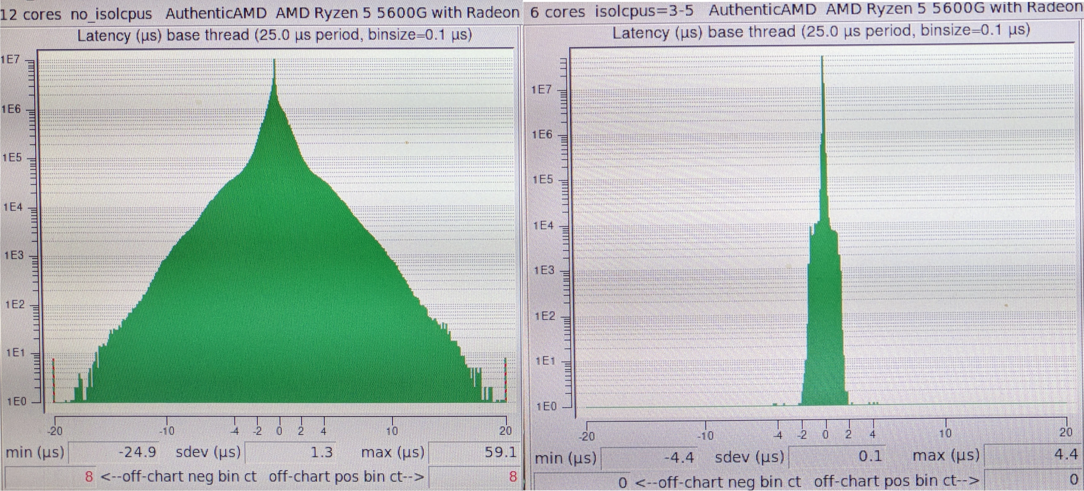 Latency & Jitter difference before (left) and after (right) Linux kernel tuning shown in histogram
Kernel preemption is the ability of kernel activities to be interrupted amid execution to switch to other higher priority tasks immediately. These can be interrupts, timers or other events.
Table of Content
- Latency and Jitter
- Preemptible Kernel Tasks
- Same Architecture Different Results
- Putting the RT in PREEMPT_RT
- Kernel Parameter Tuning
- Conclusion
- References
Latency and Jitter
But what is latency and jitter exactly and why is it important for LinuxCNC. Latency is the delay measured in time between when something is supposed to happen and when it happens (in the case of OS timers). Often times this can be accounted for assuming the delay is constant. Jitter is the variance between the delay for repeated measurements it is a measure of how constant the delay is. Jitter is much harder to correct then delay.
When using a parallel port interface, LinuxCNC needs precise timing to generate step pulses for steppers. If there is a lot of latency these step pulses will be generated to late. While if there is a lot of jitter these step pulses can become irregular.
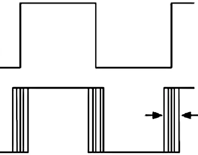 Illustrated example of jitter on step pulses, jitter free top, with jitter below
Many more modern hardware interfaces supported by LinuxCNC are much more robust against latency and jitter as the realtime and precise generation of step pulses is offloaded to dedicated hardware. Particularly the parallel port interface is very sensitive to precise timing. Most notable to the operation is that preemption can force a so called context switch between user and kernel space.
Preemptible Kernel Tasks
The job of the kernel is to switch between the many tasks and divide this work across the various components of a CPU. These tasks are known as processes while the components that do work are called cores. You can think of these cores as workers that can be assigned one task at a time$^1$. Routinely the kernel assigns one worker the task to see what everyone is doing and if it is necessary switch tasks.
This constant task switching is necessary to ensure communication with hardware such as mouse and keyboard keep working while user programs such as the browser also stay responsive. It is a delegate balance because task switching takes time. To little task switching and programs appear to stutter while to much task switching and no progress is being made so everything freezes.
Unfortunately the intervals and dynamics required for programs to feel
responsive to users is far away from being the regular interval for low latency
and low jitter. So for realtime applications the PREEMPT_RT kernel is better
suited instead. This kernel allows tasks to be interruptible at any moment in
the in case something of higher priority needs to happen part way through.
However, the results that can be expected from this kernel vary greatly depending on the exact CPU model, even if they are from the same generation and architecture!
- [1]. In reality these cores can sometimes perform multiple tasks at once in a process called Simultaneous MultiThreading (SMT).
Same Architecture Different Results
The most common desktop CPU architecture is still predominantly X86 even in 2024. Intuitively this would result in close to identical results regardless of exact CPU model but this couldn’t be further from reality. In this next section we will describe the three generations of X86 processors evaluated and discuss the latency differences.
The following three models are evaluated:
- Intel 6100U
- Intel 3770
- AMD 5600G
Of these the first model is a skylake architecture mobile processor. While the other two are a more older and newer desktop platform, respectively.
To evaluate these processors under load both glxgears and stress-ng are
used. Additional load can severely affect the results so it is needed for a
worse case measurement. In particular one instance of glxgears is started and
stress-ng is launched using --cpu N --fork N where $N$ is set to the number
of none isolated CPUs$^2$.
The test consists of a 1500 seconds run of the latency-histogram program that
is installed with the LinuxCNC package. The results including kernel tuning
are shown side by side in the following diagram.
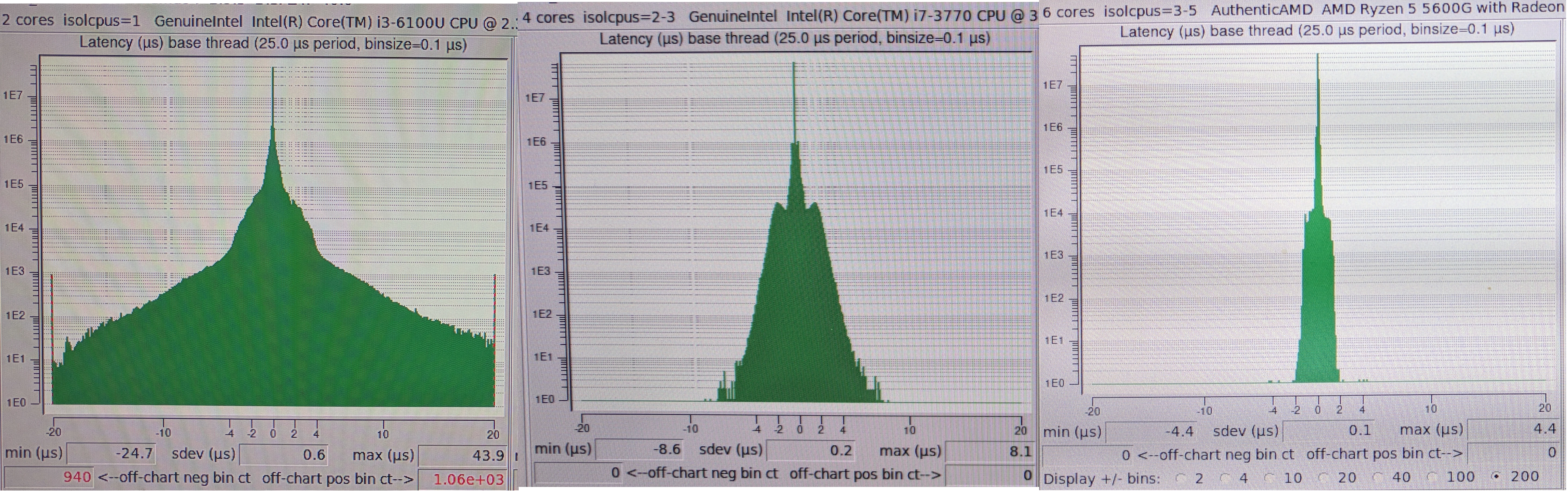 Results with kernel tuning under load for Intel i6100, Intel 3770 and AMD 5600g
Clearly, the results of the mobile platform are orders of magnitude worse then the best performing AMD desktop platform. As shown tuning does not solve these issues on all platforms. This shows that mobile X86 processors can be unfit for sensitive realtime applications and careful evaluation is needed before they are used.
- [2]. The concept of CPU isolation will be explained later.
Putting the RT in PREEMPT_RT
Linux tasks are subject to many different schedulers [1] that all exhibit
different behavior. Simply installing the PREEMPT_RT kernel will not lead to
substantially different results when running your timing sensitive programs.
For this you need to run the task with schedulers intended for realtime
applications.
On Linux there are two schedulers that are considered realtime being the fifo,
SCHED_FIFO and SCHED_RR or round-robin schedulers. These share equal
priority while already having a higher priority then regular user tasks$^3$.
The priority of these tasks is often expressed in levels between 1 and 99. Most
notably the interpreted priority for regular tasks is descending (0 being higher
priority then 99) while for RT tasks it is ascending (99 is higher then 1).
Applications like ps, top or htop often deal with this by showing the RT
task priority as a negative number.
The chrt program can be used not only to analyze but also change the scheduler
and priority of any Linux task. If you want something more modern or a bit
higher level there is also the tuna program written in Python. This section
will show examples in both.
Starting a task using a realtime scheduler requires special permissions, for
simplicity sudo is used combined with su $USER to drop back to regular
permissions. Both chrt and tuna will propagate the realtime scheduler to any
process that forks or thread that spawns from the main program.
First a new program is started using the SCHED_FIFO scheduler and priority 80:
#!/bin/bash
sudo chrt -f 80 su testuser latency-histogram
sudo tuna run -p SCHED_FIFO:80 "su testuser latency-histogram"
Next changing the scheduler to SCHED_RR and priority 40 of an already running
task using the PID without affecting children.
#!/bin/bash
sudo chrt -r --pid 40 $PID
sudo tuna priority -t $PID SCHED_RR:40
To affect all children the -a and -C options can be used on chrt and
tuna respectively.
- [3]. The remaining schedulers are
SCHED_DEADLINE,SCHED_OTHER,SCHED_IDLEandSCHED_BATCH.
The use of chrt and tuna when working with Linuxcnc is not necessary as
Linuxcnc will automatically assign the appropriate schedulers and priority to
its timing sensitive components.
Kernel Parameter Tuning
To understand the parameters for tuning one can analyze the documentation on the topic from the Linux kernel [2]. We will only briefly touch upon each parameter here.
Most importantly within Linux we can tell the kernel te reserve certain ranges or lists of cores for specific types of tasks. This allows to reserve cores for realtime tasks while simultaneously pushing hardware and os management to specific cores. The result is that we can isolate specific cores to solely run realtime tasks resulting in much better predictability in turn leading to low latency and low jitter.
The following parameters are used to push kernel threads, regular user processes
and interrupts to a subset of the cpus, here we use $N$ to denote the number of
physical processor cores the system has starting at index 0. Next we use ()
brackets to denote a mathematical formula:
irqaffinity=0-(N/2-1)kthread_cpus=0-(N/2-1)
Effectively this assigns the first half of the cores for physical tasks and interrupts. Next, we reduce the number of activities that can be assigned to the second half of the cores and isolate them for realtime tasks:
rcu_nocb_poll$^4$rcu_nocbs=(N/2)-Nnohz=onnohz_full=(N/2)-Nisolcpus=(N/2)-N
In particular the isolcpus argument reserves the cores for realtime task.
This argument needs special clarification as the value to specify depends on the
kernel version. If you use kernel 6.6 or newer it needs to be changed to
isolcpus=managed_irq,domain,(N/2)-N.
Next are a couple of arguments to prevent unpredictable execution times:
skew_tick=1, this offsets RCU timers so they do not happen at the same timenosmt=force, this disables hyperthreadingnosoftlockupnowatchdog
And lastly, we disable idle and CPU frequency adjustments as best as possible:
intel_pstate=disableamd_pstate=disableidle=pollcpufreq.off=1cpuidle.off=1intel_idle.max_cstate=1amd_idle.max_cstate=1
However, despite all these arguments, by default realtime tasks can only run for
0.95 seconds at a time before being interrupted by the kernel. While this is a
protection mechanism to prevent the system from freezing the sudden interruption
of a long running realtime task can cause jitter. Instead of controlling this
via a kernel boot argument instead it is controlled via sysfs.
sudo sysctl kernel.timer_migration=0sudo sysctl kernel.sched_rt_runtime_us=-1
This allows realtime tasks to run indefinitely, effectively till the program
calls yield or until it has to switch between user and kernel context. To
prevent manually adjusting these sysctl parameters on each boot the
/etc/sysctl.d/ directory can be used.
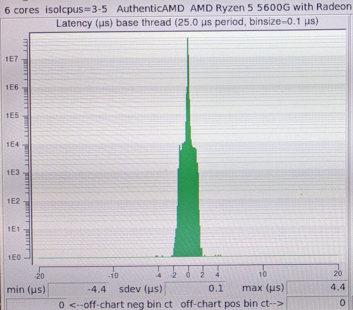 Results with kernel tuning under load for AMD 5600g
Conclusion
For reliable timing on LinuxCNC it is best to use desktop platforms that can
have boost technologies (turbo), vt-d and hardware peripherals disabled at the
bios level. Subsequent steps in modifying sysctl and kernel boot parameters
are required to even further improve timing.
The sysctl parameters in question are:
kernel.timer_migration=0
kernel.sched_rt_runtime_us=-1
While the boot parameters are:
skew_tick=1
nosmt=force
kthread_cpus=0-(N/2-1)
irqaffinity=0-(N/2-1)
rcu_nocb_poll
rcu_nocbs=(N/2)-N
nohz=on
nohz_full=(N/2)-N
isolcpus=(N/2)-N
intel_pstate=disable
amd_pstate=disable
idle=poll
cpufreq.off=1
cpuidle.off=1
intel_idle.max_cstate=1
amd_idle.max_cstate=1
nowatchdog
nosoftlockup
Be sure to adjust the ranges for N as needed. For instance on a system with
four physical cores (without hyperthreading) you would set kthread_cpus=0-1
and isolcpus=2-3.
Together these platforms and parameters allow to achieve latency in the range of 1000s of nanoseconds with jitter (in standard deviation) as low as 100 nanoseconds. An impressive achievement given the complexity of the Linux operating system running on top.
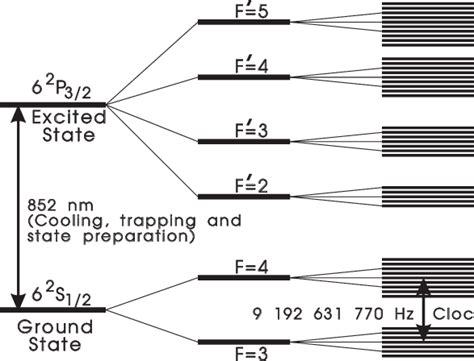 Cesium-133 atom hyperfine transition states - Bernard. J et. al. - Laser-cooled atoms and ions in precision time and frequency standards. [
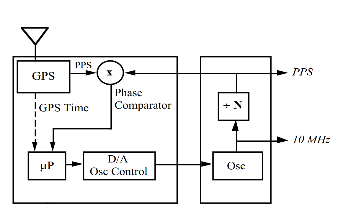 Block diagram of phase comparator controlled GPSDO
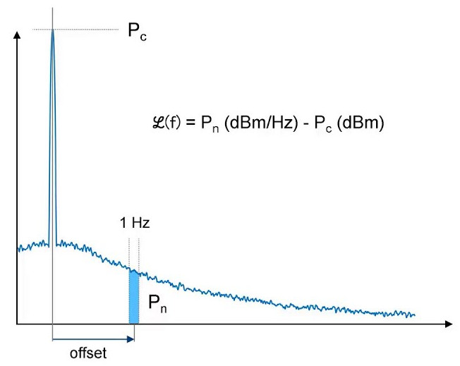 Bode plot describing how dBc/Hz is measured
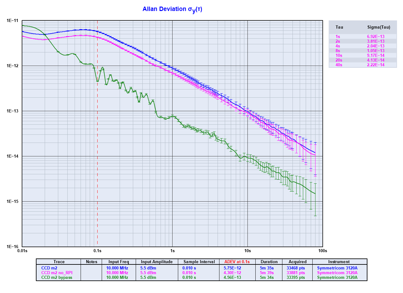 Results of OADEV calculations in TimeLab
 NanoVNA H4 and typical accessories
 Collection of General Radio GR874 Adapters & Couplers - CC BY-NC-SA 4.0 Corne Lukken (Dantali0n)
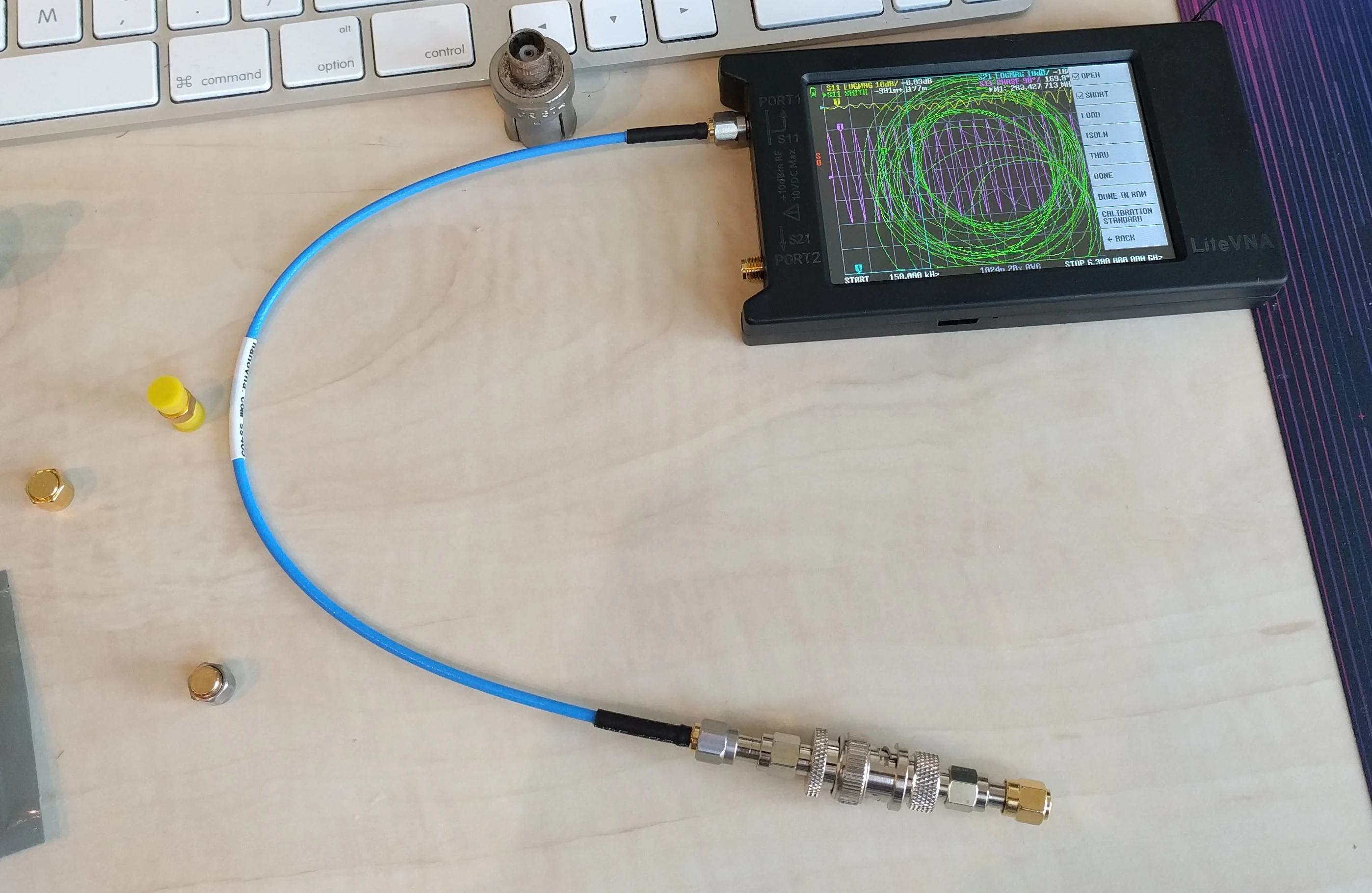 Calibration Setup for the LiteVNA - CC BY-NC-SA 4.0 Corne Lukken (Dantali0n)
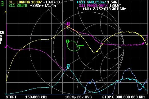 GR874 Reflections BNC male + BNC female adapters
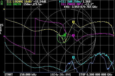 GR874 Reflections BNC male + BNC female 2nd adapter with oxide
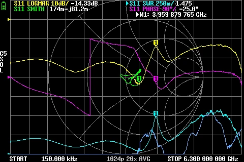 GR874 Reflections BNC male + BNC female 2nd adapter
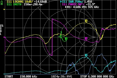 GR874 Reflections BNC male + SMA male adapter
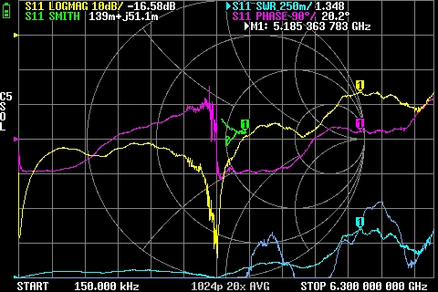 GR874 Reflections BNC male + N male adapter
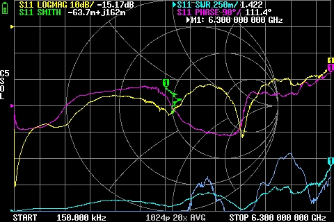 GR874 Reflections BNC male + N male 2nd adapter
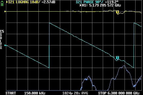 GR874 Attenuation BNC male + BNC female adapters
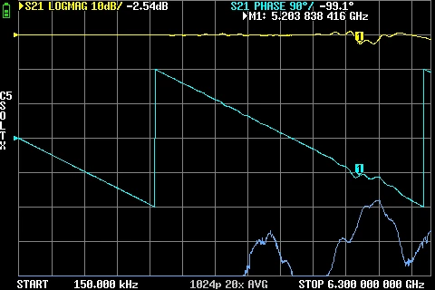 GR874 Attenuation BNC male + BNC female 2nd adapter
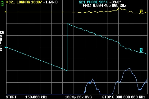 GR874 Attenuation BNC male + SMA Male
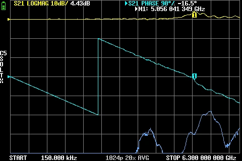 GR874 Attenuation BNC male + N Male
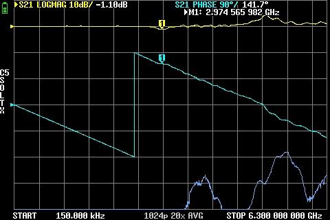 GR874 Attenuation BNC male + N Male 2nd adapter
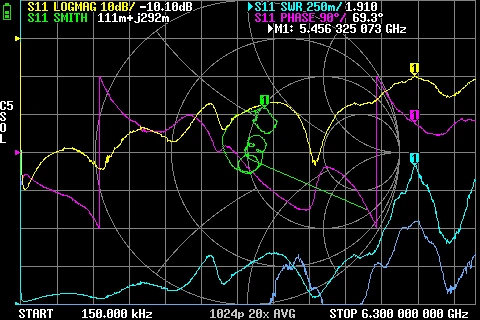 GR874 AC Coupler Reflections BNC male + SMA Male
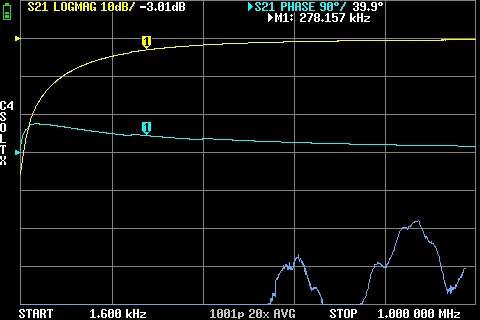 GR874 AC Coupler Attenuation Low Frequency BNC male + SMA Male
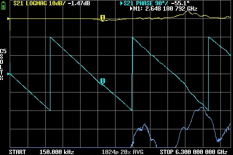 GR874 AC Coupler Attenuation BNC male + SMA Male
 Stylistic render of the Purism Librem5 - CC-by-SA
  Waydroid running on the Purism Librem5
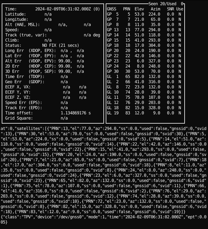 Output of CGPS in terminal
 Example STL case file rendererd